Motivation

In the rsstap Introductory vignette, we introduced the STAP formulation of models implemented using splines and demonstrated how the rsstap package uses rstan and mgcv to fit these models in a context where observations are modeled as independent of one another. In this vignette We’ll introduce the longitudinal modeling framework in rsstap that incorporates the familiar lme4 model formula syntax in addition to the between-within decomposition parameterization and syntax used to estimate between-within subject effect estimates of built environment exposure.

Simple Model

We’ll start by loading the relevant libraries and examining the included longitudinal dataset which consists of measurements on subjects “BMI” (outcome) as a function of simulated nearby “healthy food stores” (HFS) over time, similar to the longitudinal data used in the Introductory vignette:

library(rbenvo)
library(rsstap)

bdf
#> Subject Data:
#> ---------------------------:
#> Observations:  1171
#> Columns:  10
#> Num Subjects:  600
#> 
#> BEF Data:
#> ---------------------------:
#> Number of Features:  1
#> Features: 
#>   Name      Measures
#> 1  HFS Distance-Time

bef_summary(bdf)
#> # A tibble: 12 x 8
#> # Groups:   BEF, Distance_Time [2]
#>    BEF   Distance_Time Measurement  Lower Median Upper Number Num_NA
#>    <chr> <chr>               <int>  <dbl>  <dbl> <dbl>  <int>  <int>
#>  1 HFS   Distance                1 0.0261  0.487 0.974   5741      0
#>  2 HFS   Distance                2 0.0245  0.504 0.971   3524      0
#>  3 HFS   Distance                3 0.0284  0.514 0.974   1436      0
#>  4 HFS   Distance                4 0.0216  0.546 0.982    411      0
#>  5 HFS   Distance                5 0.0205  0.535 0.979     57      0
#>  6 HFS   Distance                6 0.213   0.432 0.967      9      0
#>  7 HFS   Time                    1 0.113   2.45  4.86    5741      0
#>  8 HFS   Time                    2 0.167   2.60  4.88    3524      0
#>  9 HFS   Time                    3 0.184   2.57  4.85    1436      0
#> 10 HFS   Time                    4 0.107   2.49  4.80     411      0
#> 11 HFS   Time                    5 0.148   2.56  4.89      57      0
#> 12 HFS   Time                    6 0.709   1.22  4.48       9      0

We’ll fit this model using the included sex and year covariate information, modeling the spatial temporal exposure to HFS’ through a tensor spline basis function expansion and two subject specific terms - accounting for within subject outcome correlation:

\[ E[BMI_{ij}|b_{i1},b_{i2}] = \alpha + I(Female_i)\delta_1 + (\text{year}_{ij})\delta_2 + f(\text{HFS Exposure}_{ij}) + b_{i1} + (\text{year}_{ij})b_{i2} \\\quad i = 1,...,N ; j= 1,...,n_i, \] Where \[ (b_{i1},b_{i2}) = \mathbf{b}_i \sim N(0,\Sigma), \]

akin to the standard mixed effects regression formulation as in the lme4 package and

\[ f(\text{HFS Exposure}_{ij}) = \sum_{l=1}^{L}\sum_{(d,t) \in\mathcal{S}_{ij}} \beta_l\phi_l(d,t), \]

with \(\phi_l(\cdot)\) the basis function evaluation of all relevant subject-HFS distances and times at measurement \(j\).

In order to fit this model in rsstap we can use the code below, setting the optional sampler arguments for rstan similar to how was demonstrated in the Introductory vignette.

fit <- sstap_lmer(BMI ~ sex + year + stap(HFS) + (year|ID), benvo = bdf)

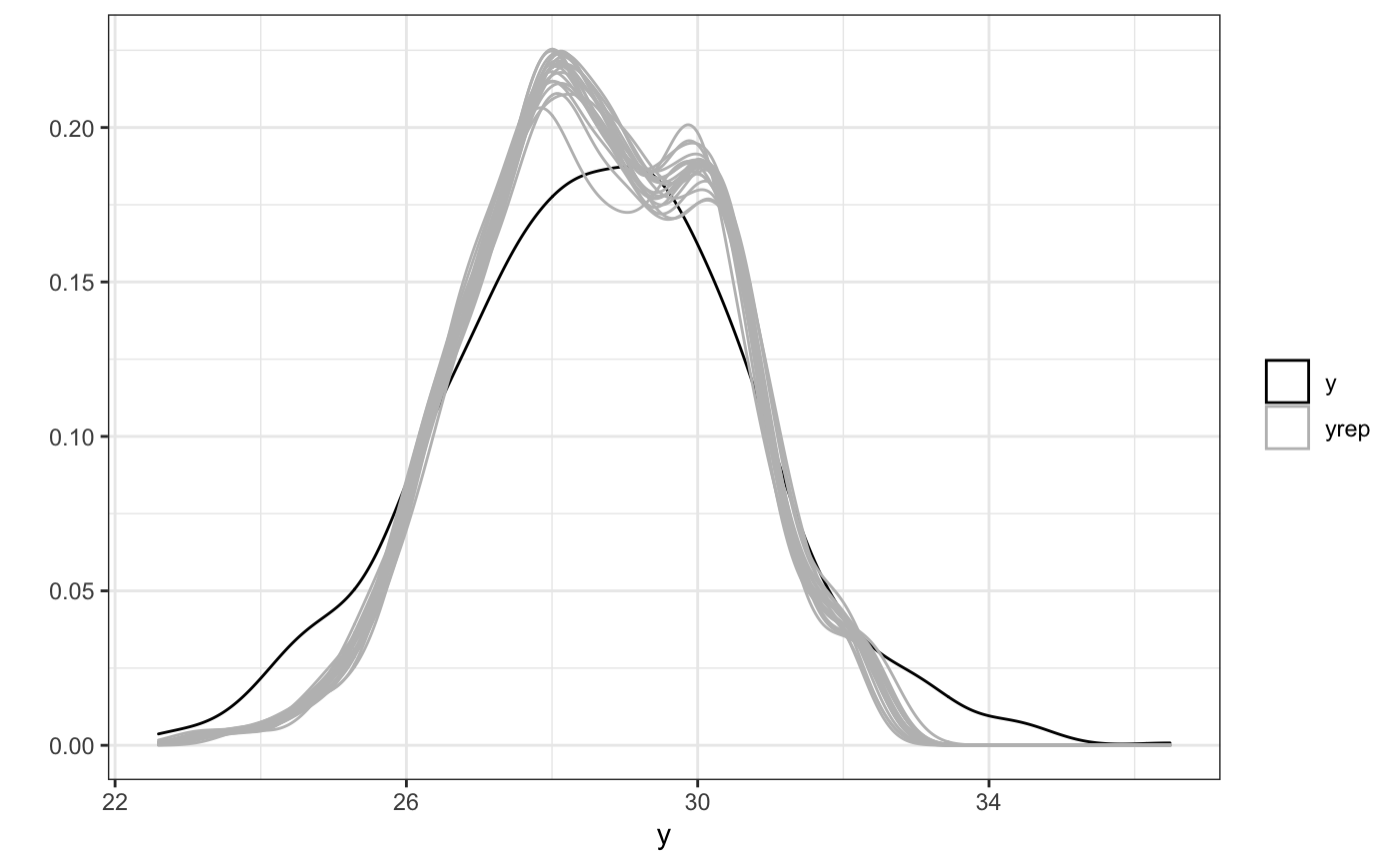
Examining the model output, we’ll first print the model quick summary followed by a graph of the posterior predictive checks to check model fit.

fit
#> 
#>  family:       gaussian [identity]
#>  formula:      BMI ~ sex + year + stap(HFS) + (year | ID)
#>  observations: 1171
#>  fixed effects:  28
#> ------
#>             Median MAD 
#> (Intercept) 32.1    0.1
#> sex         -2.2    0.1
#> year         0.1    0.0
#> t2(HFS).1    0.1    0.6
#> t2(HFS).2    0.1    0.5
#> t2(HFS).3    0.0    0.3
#> t2(HFS).4   -0.2    0.5
#> t2(HFS).5    0.1    0.4
#> t2(HFS).6   -0.4    0.3
#> t2(HFS).7    0.2    0.3
#> t2(HFS).8    0.1    0.3
#> t2(HFS).9    0.0    0.2
#> t2(HFS).10  -0.1    0.4
#> t2(HFS).11  -0.1    0.3
#> t2(HFS).12   0.0    0.2
#> t2(HFS).13  -0.3    0.5
#> t2(HFS).14  -0.2    0.4
#> t2(HFS).15   0.0    0.3
#> t2(HFS).16   0.2    0.5
#> t2(HFS).17   0.3    0.5
#> t2(HFS).18  -0.1    0.3
#> t2(HFS).19   0.3    0.4
#> t2(HFS).20   0.1    0.2
#> t2(HFS).21   0.1    0.3
#> t2(HFS).22  -0.2    0.3
#> t2(HFS).23  -0.1    0.3
#> t2(HFS).24   0.2    0.3
#> t2(HFS).25   0.1    0.3
#> 
#> Smoothing terms:
#>                            Median MAD_SD
#> smooth_precision[t2(HFS)1] 2.9    1.5   
#> smooth_precision[t2(HFS)2] 2.6    1.4   
#> smooth_precision[t2(HFS)3] 2.4    1.3   
#> smooth_precision[t2(HFS)4] 2.1    1.3   
#> 
#> Error terms:
#>  Groups   Name        Std.Dev. Corr  
#>  ID       (Intercept) 0.16774        
#>           year        0.29006  -0.244
#>  Residual             1.19162        
#> Num. levels: ID 600

ppc(fit)

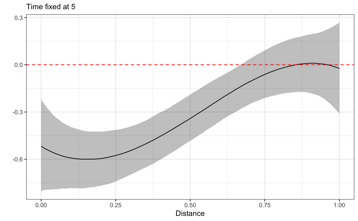
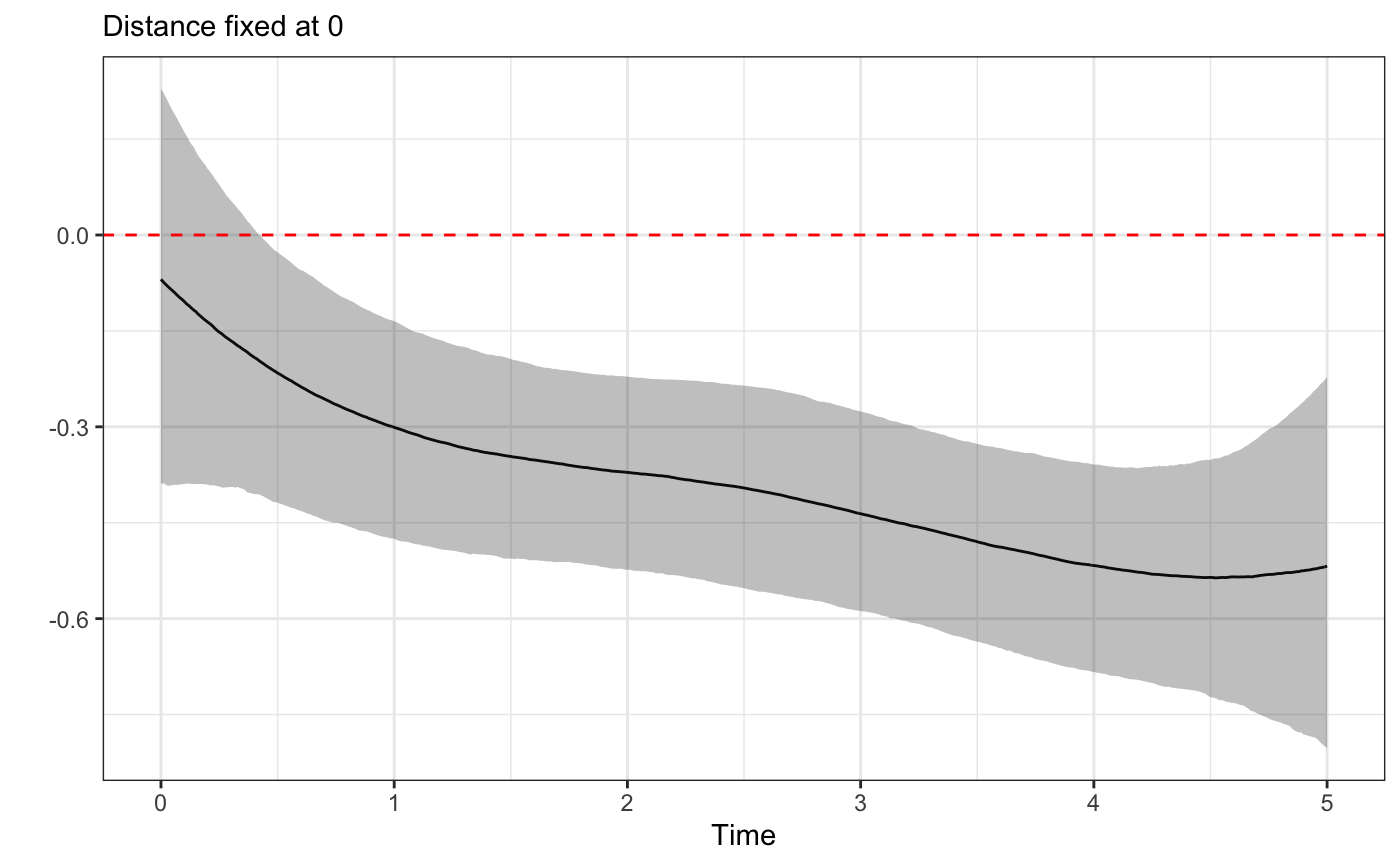
Finally we’ll look at a 3d plot and 2d plot cross sections of the HFS effect across space and time. This will allow us to establish whether there is any effect at all, and what it looks like.

plot3D(fit)

plot_xsection(fit,fixed_val=5)

plot_xsection(fit,component = "Time",fixed_val=0)

The Missing Piece

The model ran and converged successfully and the output looks meaningfully interesting! But there’s something important we forgot to take into account. With time-varying covariates, such as age, income, etc. It is important to decompose the measure into the baseline or between-subject effect and the change, or within-subject effect as these each represent two different effects. Failing to decompose these time-varying measures can result in invalid inference!(Nehaus and Kalbfleisch 1998)

Between-Within Decomposition, Interpretation

There are a number of ways this decomposition could be be obtained. In the rsstap model the decomposition takes the following form (keeping all other components the same as in the previous model):

\[ E[BMI_{ij}|b_{i1},b_{i2}] = \alpha + I(Female_i)\delta_1 + (\text{year}_{ij})\delta_2 + \Delta f(\text{HFS Exposure}_{ij}) + \bar{f}(\text{HFS Exposure}_{i}) + b_{i1} + (\text{year}_{ij})b_{i2} \\\quad i = 1,...,N ; j= 1,...,n_i, \] Where \[ \bar{f}(HFS_i) = \sum_{j=1}^{n_i} \sum_{(d,t) \in \mathcal{S}} \sum_{l=1}^{L} \beta_l \phi_l(d,t)\\ \Delta f(HFS_i) = \sum_{(d,t) \in \mathcal{S}} \sum_{l=1}^{L} \beta_l \phi_l(d,t) - \bar{f}(HFS_i). \\ \]

This allows our spatial-temporal effect estimate of HFS exposure to be separated into an average exposure (between subject) effect and a deviation from average (within subject) effect. The latter of these two is a difference in difference estimator, which - through its differencing - controls for unobserved time-invariant confounders. If we included the relevant time varying confounders in our model, e.g. Age, income, education, etc. and the usual causal inference identifiability conditions hold, then our estimate \(\Delta f(\cdot)\) has a causal interpretation!

We’ll fit this model below, using the rsstap syntax that requires a _bw after the usual stap,sap, or tap function designation and running the same model diagnostics as before.

bw_fit <- sstap_lmer(BMI ~ sex + stap_bw(HFS) + (year|ID), benvo = bdf)

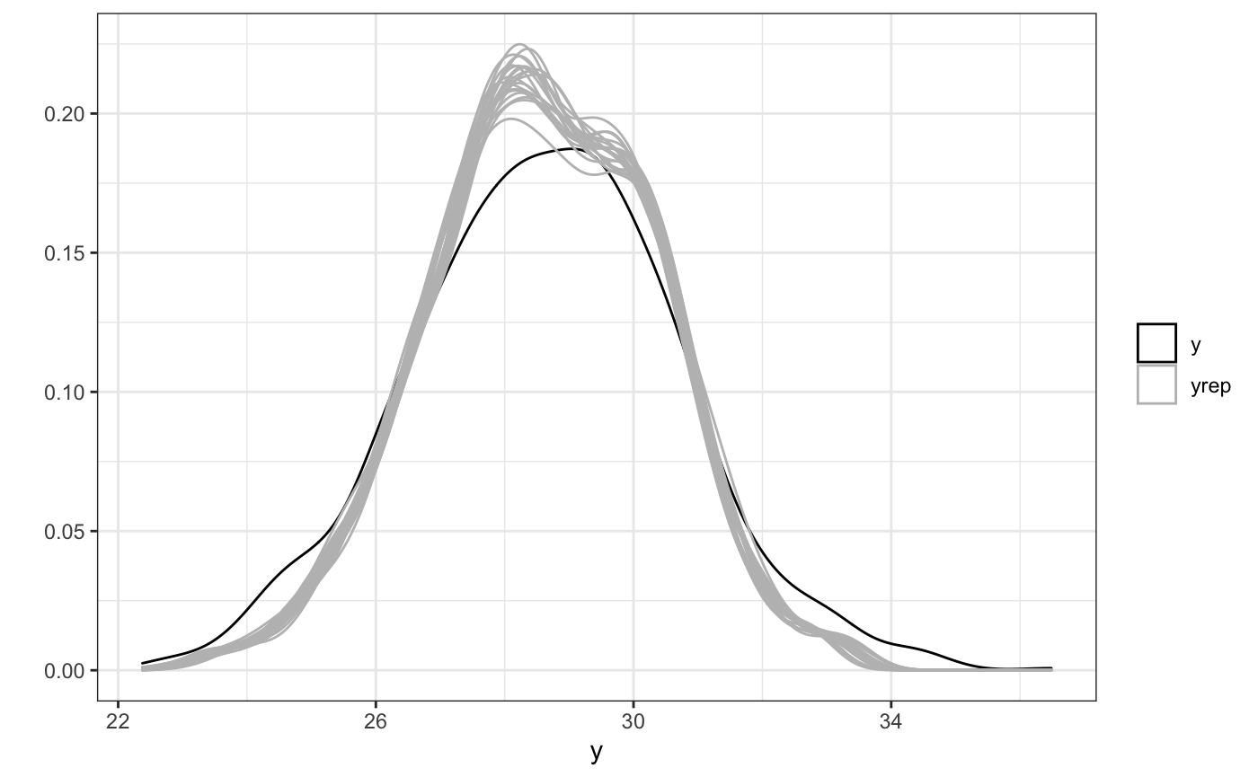
ppc(bw_fit)

Now that we’re estimating two effects, we can look at two different 3D plots of the HFS effect. These are contained in a list from the plot3D output, labeled intuitively as you’ll see.

plts <- plot3D(bw_fit)

plts$Between

In the between-subject effect plot, we see that for an increase in average exposure to HFS’, we would expect an appreciable decrease in the average BMI.

plts$Within

In the above plot, we can see that for changes in an individual subject’s average exposure to HFS, their BMI decreases - not as much as it does for an average increase in exposure, as in the previous plot, but a negative effect all the same.

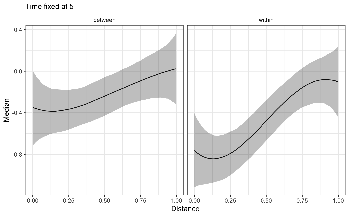
Similarly, and perhaps more easily to visualize, we can plot cross sections of the functions, fixing the maximum (minimum) time (distance) and plotting the corresponding spatial (temporal) function.

plot_xsection(bw_fit,fixed_val=5)

plot_xsection(bw_fit,component="Time",fixed_val=0)

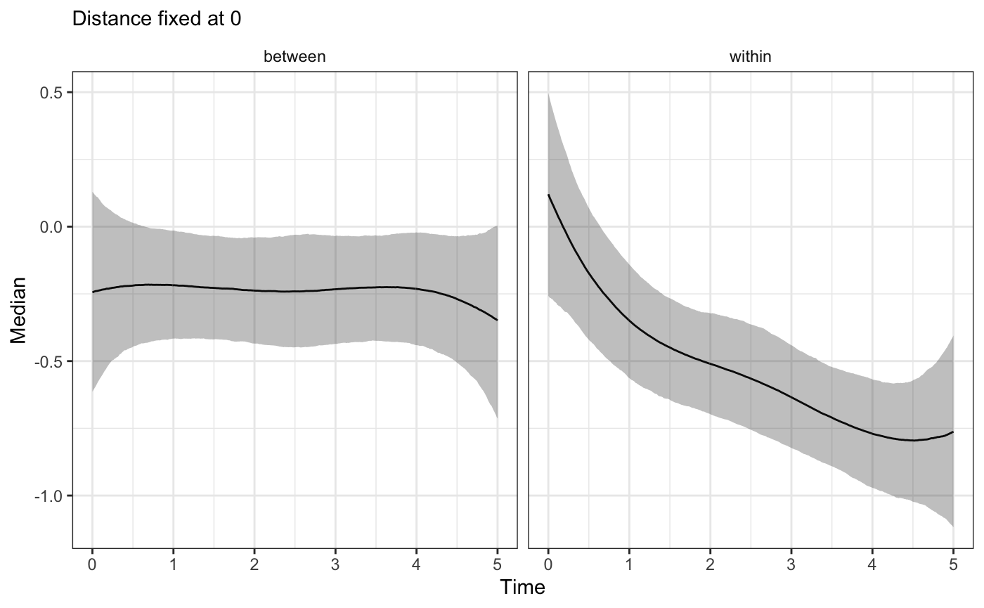
As all these plots show, we observe two, different effects from HFS exposure over time! In a real world scenario this difference will be important for the substantive understanding of the HFS impact on subject health.

Summary

In summary, a scientist interested in examine the built environment needs longitudinal data gathered over time to really get a greater sense of whether or not exposure to the built environment feature (BEF) of interest has any meaningful effect on subjects’ health. In constructing those models it is important to do so with a decomposition of the non-linear BEF exposure effect into between-within components, both to avoid bias and improve understanding!

References

Nehaus, John, and Jack Kalbfleisch. 1998. “Between-and Within-Cluster Covariate Effects in the Analysis of Clustered Data.” Biometrics, June, 638–45. https://doi.org/10.2307/3109770.