Motivation
The rstap package introduced Spatial Temporal Aggregated Predictor or STAP models, as a method by which the effect of Built Environment Features (BEFs) measured as a point pattern could be incorporated into pre-existing regression methods. The rsstap package builds on this framework by modifying the way in which the spatial temporal exposure effect is estimated. We’ll begin this demonstration by loading the relevant libraries, before getting into the modelling notation and code examples.
Model Specification
Restricting our attention to only spatial exposure for the following illustrative example, the spatial aggregated predictor both rstap and rsstap fit models of the following form:
\[ E[g(\mu_i)] = Z_i^{T}\delta + f(\mathcal{D}_i) \quad i=1,...,n \]
While link function \(g(\cdot)\), univariate mean \(\mu_i\) and covariates \(Z_i\) for subject \(i=1,...,n\) are identified from a typical regression model, the function \(f(\mathcal{D}_i)\) novelly represents the \(i\)th subject’s cumulative exposure across space. In rstap This was accomplished by incorporating distances, \(d\) through a spatial exposure function \(f(\mathcal{D}_i) = \sum_{d \in \mathcal{D}_i} \mathcal{K}_s(d,\theta)\) - typically some exponential decay function, like \(\exp(-\frac{d}{\theta})\) or \(\exp(-(\frac{d}{\theta})^{\eta})\). Unfortunately, estimating this model through standard methods (e.g. MCMC) requires numerous evaluations of the kernel function summed across the, again typically numerous, distances in the sets \(\mathcal{D}_i\) , of subject-BEF distances.
To remedy this situation, the rsstap package adopts a regression spline basis representation, \(f(d) = \sum_{j=0}^{J} \beta_j\phi_j(d)\), of the spatial exposure effect, removing the kernel and allowing for estimation on a sum of the function of the distances:
\[ E[g(\mu_i)] = Z_i^{T}\delta + \sum_{j=0}^{J}\sum_{d \in \mathcal{D}_i}\beta_j\phi_j(d) \]
Since the sum across distances, \(\sum_{d\in \mathcal{D}_i} \phi_j(d)\) can be done prior to model fitting, standard methods (essentially a bayesian equivalent to mgcv::gam) can be used, dramatically decreasing computational complexity. Specifically, we use the No U-Turn sampler variant available via rstan for full bayesian inference of the posterior distribution of these functional terms. Finally, information about priors for rsstap models can be found here.
Illustration
We’ll illustrate this using a simple dataset that contains outcome BMI as a function of a binary covariate sex and simulated fast food restaurant (FFR) exposure. These data are contained in the benvo package.
As can be seen below, the model formula and syntax are akin to the typical lm function, with the addition of a sap(FFR) term to represent the fact that we’ll be modelling FFR exposure as a spatial aggregated predictor. Let’s fit this model using the standard sampling defaults of 2000 samples drawn from 4 independent chains, using the first 1000 from each as burn-in.
fit <- sstap_lm(BMI ~ sex + sap(FFR),
                example_benvo)
We’ll examine the model fit by first looking at a print out summary of the model followed by the posterior predictive checks - a basic model check tool.
fit
#>
#>  family:       gaussian [identity]
#>  formula:      BMI ~ sex + sap(FFR)
#>  observations: 1000
#>  fixed effects:  12
#> ------
#>             Median MAD
#> (Intercept) 25.9    0.1
#> sex         -2.1    0.1
#> s(FFR).1     3.1    0.9
#> s(FFR).2     2.9    0.1
#> s(FFR).3     3.1    0.1
#> s(FFR).4     2.9    0.1
#> s(FFR).5     2.7    0.1
#> s(FFR).6     1.4    0.1
#> s(FFR).7     0.1    0.1
#> s(FFR).8     0.0    0.1
#> s(FFR).9    -0.1    0.1
#> s(FFR).10    0.7    0.9
#>
#> Smoothing terms:
#>                           Median MAD_SD
#> smooth_precision[s(FFR)1] 4.0    1.8
#> smooth_precision[s(FFR)2] 0.1    0.1
ppc(fit)
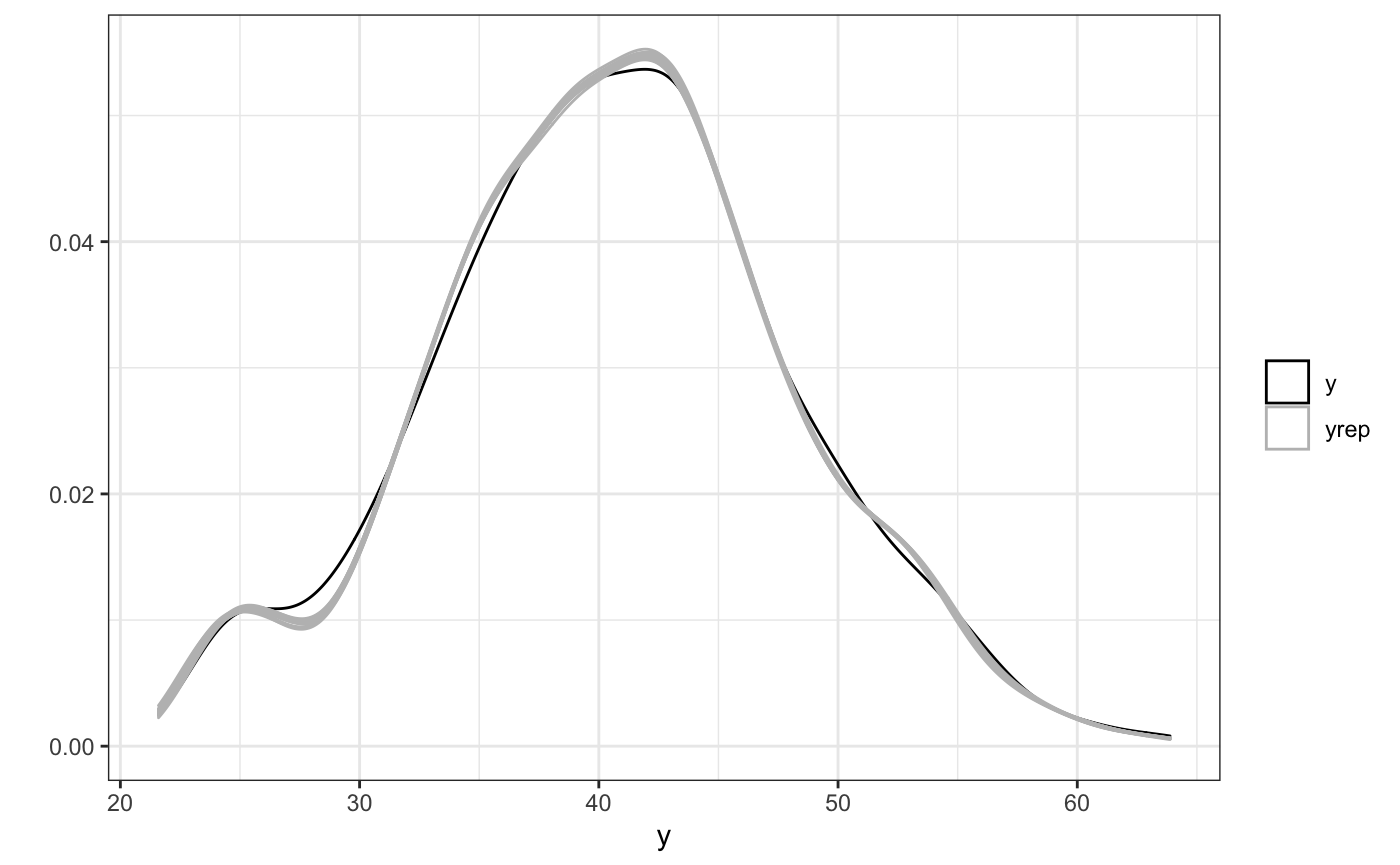
Next we’ll take a look at the spatial effect of one single FFR on the expected BMI of subjects as a function of space. We’ll overlay the true function (since this is simulated data) in red on top.
plot(fit) + truth
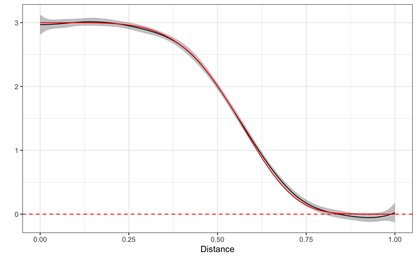
While the curves won’t always be so well defined, this example illustrates the basics of fitting stap models using the spline implimentation via rsstap. The next section will go through the basics of spatial-temporal estimation without adjusting for within subject correlation.
Longitudinal Spatio-Temporal example
In this quick example, we’ll briefly run through the same function calls as before, now using a longitudinal simulated dataset that contains both spatial and temporal data. Note that while a longitudinal model should take into account correlation across a given subject’s measurements, we’ll stick to the simpler model now for exposition (see the longitudinal vignette for how to account for these terms). Let’s first look at the longitudinal_HFS data that comes with the rsstap package, renamed here as bdf2 for brevity.
bdf2
#> Subject Data:
#> ---------------------------:
#> Observations:  596
#> Columns:  6
#> Num Subjects:  300
#>
#> BEF Data:
#> ---------------------------:
#> Number of Features:  1
#> Features:
#>   Name      Measures
#> 1  HFS Distance-Time
Looks like this data contains 300 subjects with both distances and times measured for the subjects. In order to fit the same kind of model as before, but now taking into account both space and time, we’ll use the stap designation in the model formula. This is equivalent to using the t2 spline basis expansion from mgcv.
fit <- sstap_lm(BMI ~ sex + stap(HFS), benvo = bdf2)
#> Warning in check_for_longitudinal_benvo(benvo): This Benvo was constructed with longitudinal data
#>  but sstap_lm does not adjust for within subject correlation.
#>  Be advised that parameter standard errors may be overoptimistic.
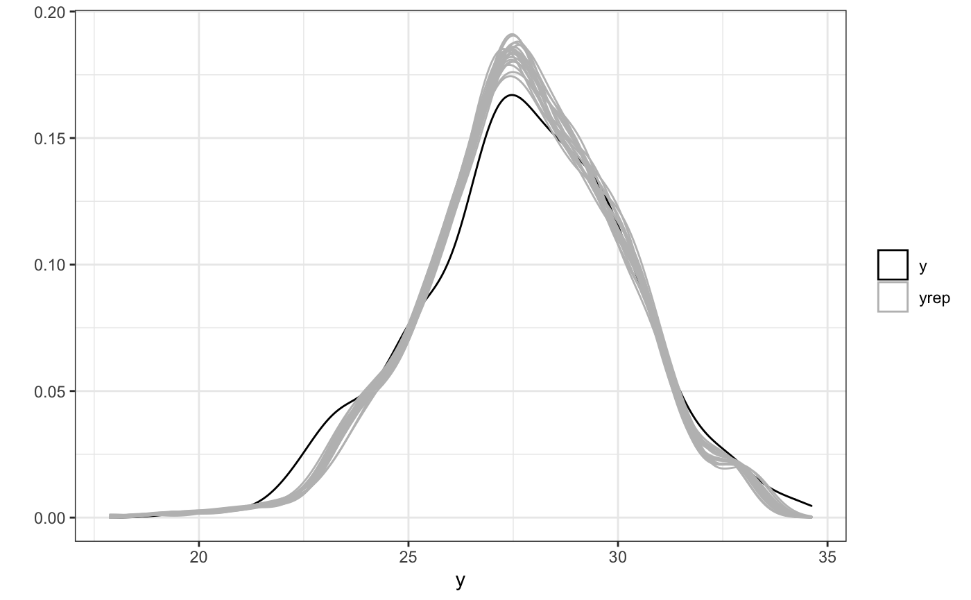
We’ll examine the posterior predictive checks first to verify that indeed the model can recover the true simulated parameters.
ppc(fit)
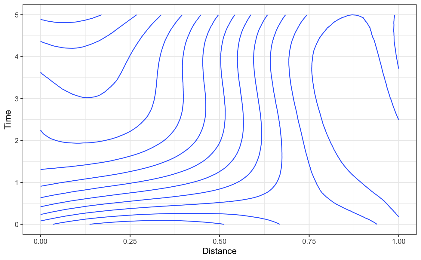
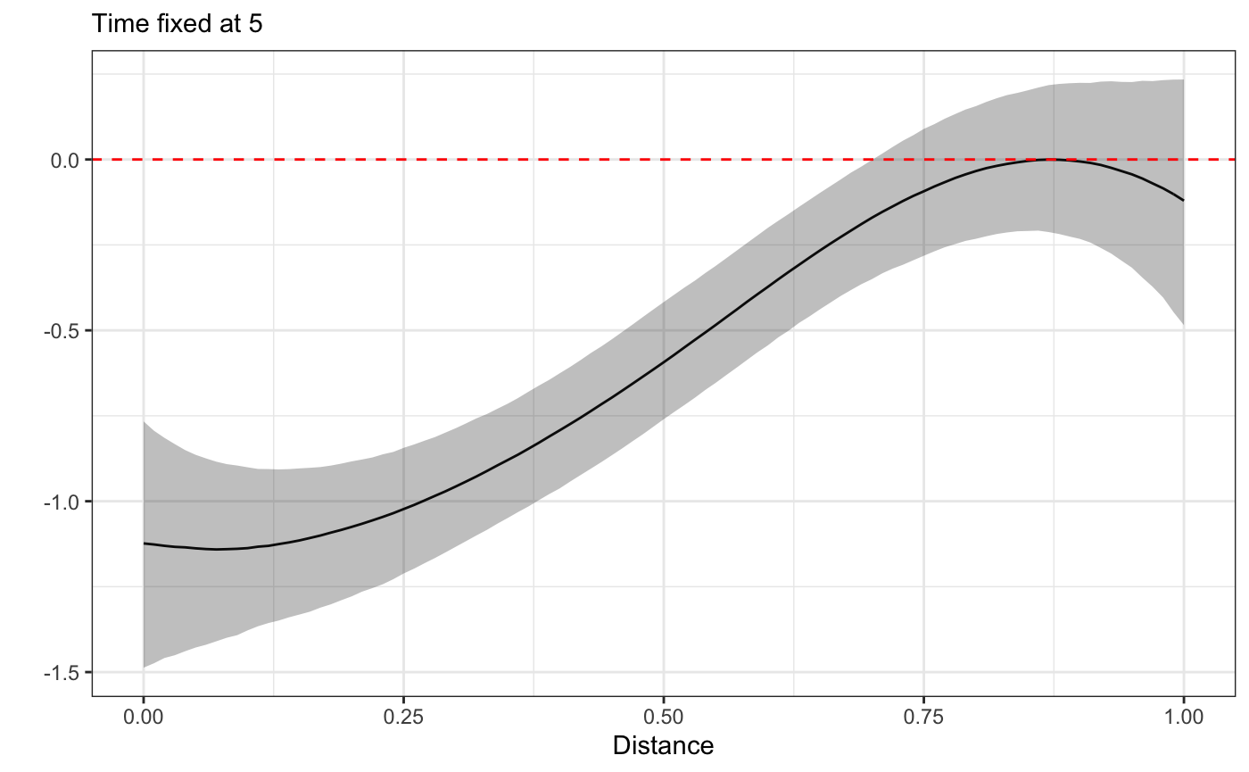
Then, onto the spatio-temporal effects. Calling the plot method on this fitted object will produce a contour plot. rsstap also provides a plot_xsection which plots the cross section of the surface at a fixed value and a plot3D function via the rplotly package that can plot the surface in 3 dimensions.
plot(fit)
plot_xsection(fit,fixed_val=5)
plot3D(fit)
With both spatial and spatio-temporal model-fitting now demonstrated, it is our hope that you have a greater familiarity of some of the basics of rsstap and the STAP modeling framework.
Advanced Topics
This concludes the introductory vignette. With built environment - subject data, the rsstap package can be used to estimate how nearby built environment features may effect the outcome of interest via the STAP modeling framework.
See the other vignettes for elaborations on the spline implementation of spatial temporal aggregated predictors in a longitudinal context, wherein subject specific and between/within effects are estimated as well as so-called “network effects” of BEFs .