library(rbenvo)
Motivation
In the Introductory vignette, the benvo class was introduced using subject and built environment feature (BEF) data that had already been joined and calculated. An alternative way to construct benvo’s (as of v1.0.0) is to calculate the distances and times from the Subject and BEF data iteratively. This requires that the data be stored either as an sf object for distance calculation and/or there be date/time information. In this vignette, I’ll demonstrate how to program this iterative construction beginning with an example where there is spatial data, covering temporal data subsequently.
Spatial Data
We’ll begin with a look at two datasets composed of subject and BEF data respectively that can be procured publicly via the California Department of Education and the osmdata package respectively (See here for how I downloaded these data). The former dataset contains information on 5th, 7th and 9th graders’ obesity at schools through the state of California, though we’ll focus on those schools and restaurants in Los Angeles for ease of exposition.
LA_schools
#> # A tibble: 698 x 9
#>    cdscode Charter Grade     N Percent NoStud_Overweig… NoStud_NotOverw…
#>    <chr>   <fct>   <fct> <dbl>   <dbl>            <dbl>            <dbl>
#>  1 141014… Charter 9        19    47.4                9               10
#>  2 191019… Charter 7        92    35.9               33               59
#>  3 191019… Charter 9        44    52.3               23               21
#>  4 191019… Tradit… 9        99    19.2               19               80
#>  5 196473… Charter 5        45    33.3               15               30
#>  6 196473… Charter 5       101    59.4               60               41
#>  7 196473… Charter 7       127    59.4               75               52
#>  8 196473… Charter 5       101    46.5               47               54
#>  9 196473… Charter 7       127    46.5               59               68
#> 10 196473… Charter 5        65    46.2               30               35
#> # … with 688 more rows, and 2 more variables: Latitude <dbl>, Longitude <dbl>
The latter dataset contains businesses labeled as “Fast Food” in the Los Angeles Area, by users of openstreetmap, a crowd-sourcing map tool which allows users to document different areas of their environment.
LA_FF
#> # A tibble: 6,621 x 4
#>    Name               osm_id    Latitude Longitude
#>    <chr>              <chr>        <dbl>     <dbl>
#>  1 <NA>               60713740     -118.      34.1
#>  2 Yoshinoya          72448982     -118.      34.1
#>  3 Jack in the Box    72448995     -118.      34.1
#>  4 Baja Fresh         344723703    -118.      34.2
#>  5 Jersey Mike's Subs 344723888    -118.      34.2
#>  6 Taco Bell          344727689    -118.      34.2
#>  7 Baja Fresh         349339405    -118.      34.1
#>  8 Chipotle           349340479    -118.      34.1
#>  9 Subway             354910320    -118.      34.3
#> 10 <NA>               358019457    -118.      34.2
#> # … with 6,611 more rows
In order to prepare these data for use in a benvo, we’ll convert them to sf objects using the sf::st:as_sf() function as follows. Note that while these data are sfc_POINT objects, they could be any sf object, provided they have a location and a measure of distance can be calculated between the subject and bef data frames.
To create a benvo, we use the same benvo() function as used with pre-calculated data, but we now specify the unique subject id so the object can correctly link future data tables.
benvo(LA_schools,by='cdscode')
#> Active df:  subject
#> Simple feature collection with 698 features and 7 fields
#> geometry type:  POINT
#> dimension:      XY
#> bbox:           xmin: -118.4958 ymin: 33.90556 xmax: -118.136 ymax: 34.29046
#> geographic CRS: WGS 84
#> # A tibble: 698 x 8
#>    cdscode Charter Grade     N Percent NoStud_Overweig… NoStud_NotOverw…
#>  * <chr>   <fct>   <fct> <dbl>   <dbl>            <dbl>            <dbl>
#>  1 141014… Charter 9        19    47.4                9               10
#>  2 191019… Charter 7        92    35.9               33               59
#>  3 191019… Charter 9        44    52.3               23               21
#>  4 191019… Tradit… 9        99    19.2               19               80
#>  5 196473… Charter 5        45    33.3               15               30
#>  6 196473… Charter 5       101    59.4               60               41
#>  7 196473… Charter 7       127    59.4               75               52
#>  8 196473… Charter 5       101    46.5               47               54
#>  9 196473… Charter 7       127    46.5               59               68
#> 10 196473… Charter 5        65    46.2               30               35
#> # … with 688 more rows, and 1 more variable: geometry <POINT [°]>
In order to construct the new table of subj-BEF distances and incorporate the bef table into the relational data structure of the benvo, the appropriately named add_BEF() function works much like it sounds. We can then activate the restaurant table in order to look at the distances.
benvo(LA_schools,by='cdscode') %>%
  add_BEF(FFR,bef_id = 'osm_id') %>%
  activate(FFR) -> bdf
#> Linking to GEOS 3.8.1, GDAL 3.1.1, PROJ 6.3.1
bdf
#> Active df:  FFR
#> # A tibble: 4,621,458 x 3
#>    cdscode        osm_id    Distance
#>    <chr>          <chr>          [m]
#>  1 14101400128454 60713740 19717.047
#>  2 19101990134361 60713740 17167.510
#>  3 19101990135582 60713740 17606.308
#>  4 19101991933399 60713740  5907.847
#>  5 19647330100289 60713740  9887.820
#>  6 19647330100669 60713740 18522.629
#>  7 19647330100669 60713740 18522.629
#>  8 19647330100669 60713740 18522.629
#>  9 19647330100669 60713740 18522.629
#> 10 19647330100743 60713740 14184.749
#> # … with 4,621,448 more rows
As can be seen here, the add_BEF() function uses the sf::st_distance function by default which returns a distance (great circle distance in this case) according to the coordinate reference system set for the sf objects. In this case the units are meters , but we can convert them to km and remove those pairings that are greater than 10km using the dplyr verbs adapted to function on whatever table is currently active in the benvo. Since we have repeat measurements for each school we have multiple distances for each school when we only need 1, so we’ll use a combination of filter and distinct to remove the duplicate and extraneous (>10 km) distances:
bdf <- bdf %>%
  mutate(Distance = as.numeric(Distance/1E3)) %>%
  filter(Distance<=10) %>%
  distinct(cdscode,osm_id,Distance)
bdf
#> Active df:  FFR
#> # A tibble: 489,034 x 3
#>    cdscode        osm_id   Distance
#>    <chr>          <chr>       <dbl>
#>  1 19101991933399 60713740     5.91
#>  2 19647330100289 60713740     9.89
#>  3 19647330100867 60713740     9.55
#>  4 19647330101683 60713740     5.48
#>  5 19647330102426 60713740     6.37
#>  6 19647330106435 60713740     9.36
#>  7 19647330108886 60713740     7.89
#>  8 19647330109439 60713740     3.22
#>  9 19647330110304 60713740     8.82
#> 10 19647330111658 60713740     5.91
#> # … with 489,024 more rows
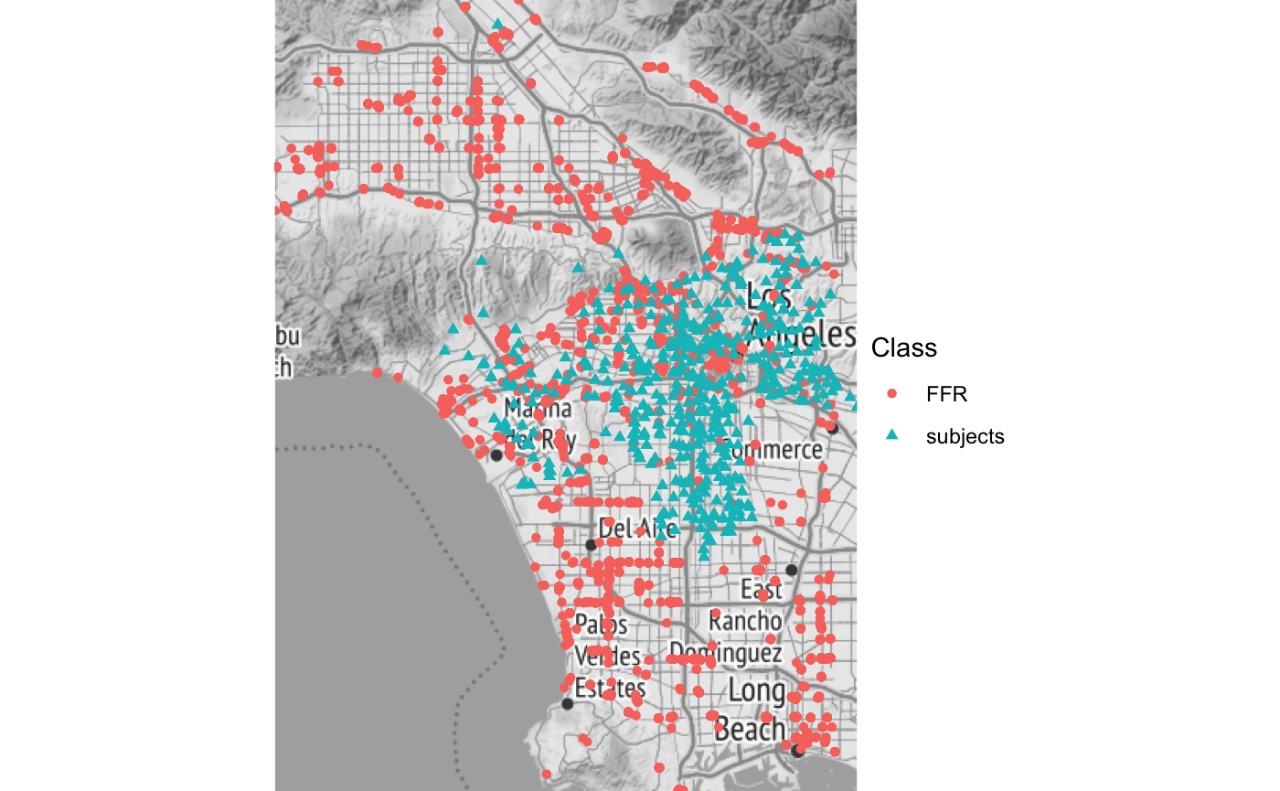
While we could get a sense of the distribution of distances using the plot_pointrange() function as illustrated in the Introductory vignette, instead, here we’ll use the plot_map() function, via the plot which will produce a ggplot object of the spatial objects distinguished as BEF or subject by color on a map defined by the boundaries of the combined sf objects, using ggmap to request the underlying stamen map.
plot(bdf,'map') + ggplot2::theme_bw() + ggplot2::theme_void()
#> Source : http://tile.stamen.com/terrain/10/174/407.png
#> Source : http://tile.stamen.com/terrain/10/175/407.png
#> Source : http://tile.stamen.com/terrain/10/174/408.png
#> Source : http://tile.stamen.com/terrain/10/175/408.png
#> Source : http://tile.stamen.com/terrain/10/174/409.png
#> Source : http://tile.stamen.com/terrain/10/175/409.png
#> Coordinate system already present. Adding new coordinate system, which will replace the existing one.
 For more on how these data might be modeled, check out the
 rsstap or bentobox packages.
Having looked at how benvo’s handle spatial data, we’ll now turn to temporal data.
Temporal Data
Similar to how one may have spatial data available for built environment features and subjects it’s also possible to have temporal data, describing the time a subject spent at a specific location. Depending on the analysis spatial and temporal structures can both be quite complex, as before we’ll illustrate how temporal data can be incorporated into a benvo with cross-sectional temporal data where each subject is only associated with one time point. More complex temporal data, where there are multiple time points associated with each subject, as in the case of longitudinal data, will be incorporated in a future release.
Temporal Data Simulation
We’ll begin by simulating dates for the Los Angeles Schools that have fifth graders and Fast Food Restaurant data. We’ll set all schools to start sometime in the fall, and have the business arbitrarily open and close sometime after 2015.
set.seed(342431)
LA_schools_five  <-  LA_schools %>% filter(Grade==5)
origin <- lubridate::as_date("2018-08-01")
school_start <- origin+sample(1:120,size = nrow(LA_schools_five),replace = TRUE)
measure_date <- lubridate::as_date("2019-05-01")
close_date <- measure_date
business_start_date <- origin + sample(-786:786,size = nrow(LA_FF),replace = TRUE)
business_close_date <- business_start_date + sapply((lubridate::today()-business_start_date),function(x) sample(1:x,1))
FFR <- LA_FF %>%
  mutate(open=business_start_date,close=business_close_date)
schools <- LA_schools_five %>% mutate(open=school_start,measure=measure_date,close=close_date)
We create the benvo using the same function as before, but now including the optional arguments that specify the start,measurement, and stop date columns for each subject observation which are each vectors of lubridate::Date objects. These must be named similarly in any subsequent BEF table that is then added, as in the FFR example here. The benvo() function uses these date columns to then construct the time exposed, labeled as Time and exposure lag (time between the end of the exposure period and the current measurement date)
bdf <- benvo(schools,
      start_date_col="open",
      measurement_date="measure",
      stop_date_col="close",by='cdscode') %>%
  add_BEF(FFR,bef_id = 'osm_id')
We can look at the constructed times, by activating the FFR table.
bdf %>% activate(FFR) %>%
  select(-open,-close) ## for better display
#> Active df:  FFR
#> # A tibble: 1,187,983 x 7
#>    cdscode       measure    open_FFR   close_FFR  osm_id    Time    exposure_lag
#>    <chr>         <date>     <date>     <date>     <chr>     <drtn>  <drtn>
#>  1 196473301002… 2019-05-01 2016-06-06 2019-10-05 41070726… 157 da…  0 days
#>  2 196473301002… 2019-05-01 2016-06-07 2019-05-24 38614490… 157 da…  0 days
#>  3 196473301002… 2019-05-01 2016-06-08 2020-08-15 46611260… 157 da…  0 days
#>  4 196473301002… 2019-05-01 2016-06-09 2019-04-29 42256375… 155 da…  2 days
#>  5 196473301002… 2019-05-01 2016-06-09 2019-07-18 44859943… 157 da…  0 days
#>  6 196473301002… 2019-05-01 2016-06-09 2020-01-02 43124339… 157 da…  0 days
#>  7 196473301002… 2019-05-01 2016-06-09 2020-10-15 37616364… 157 da…  0 days
#>  8 196473301002… 2019-05-01 2016-06-10 2019-03-10 46601780… 105 da… 52 days
#>  9 196473301002… 2019-05-01 2016-06-10 2019-05-17 43027016… 157 da…  0 days
#> 10 196473301002… 2019-05-01 2016-06-11 2019-02-01 40901984…  68 da… 89 days
#> # … with 1,187,973 more rows
Similar to how the distances were calculated in specific units from the sf::st_distance() function, the lubridate function calculates differences in times according to the granularity of the data. Here since we have information available in days, we calculate differences in units of days. These can be altered according to user preference, as before using the dplyr verb functions and converting times according to the functions in the lubridate package.
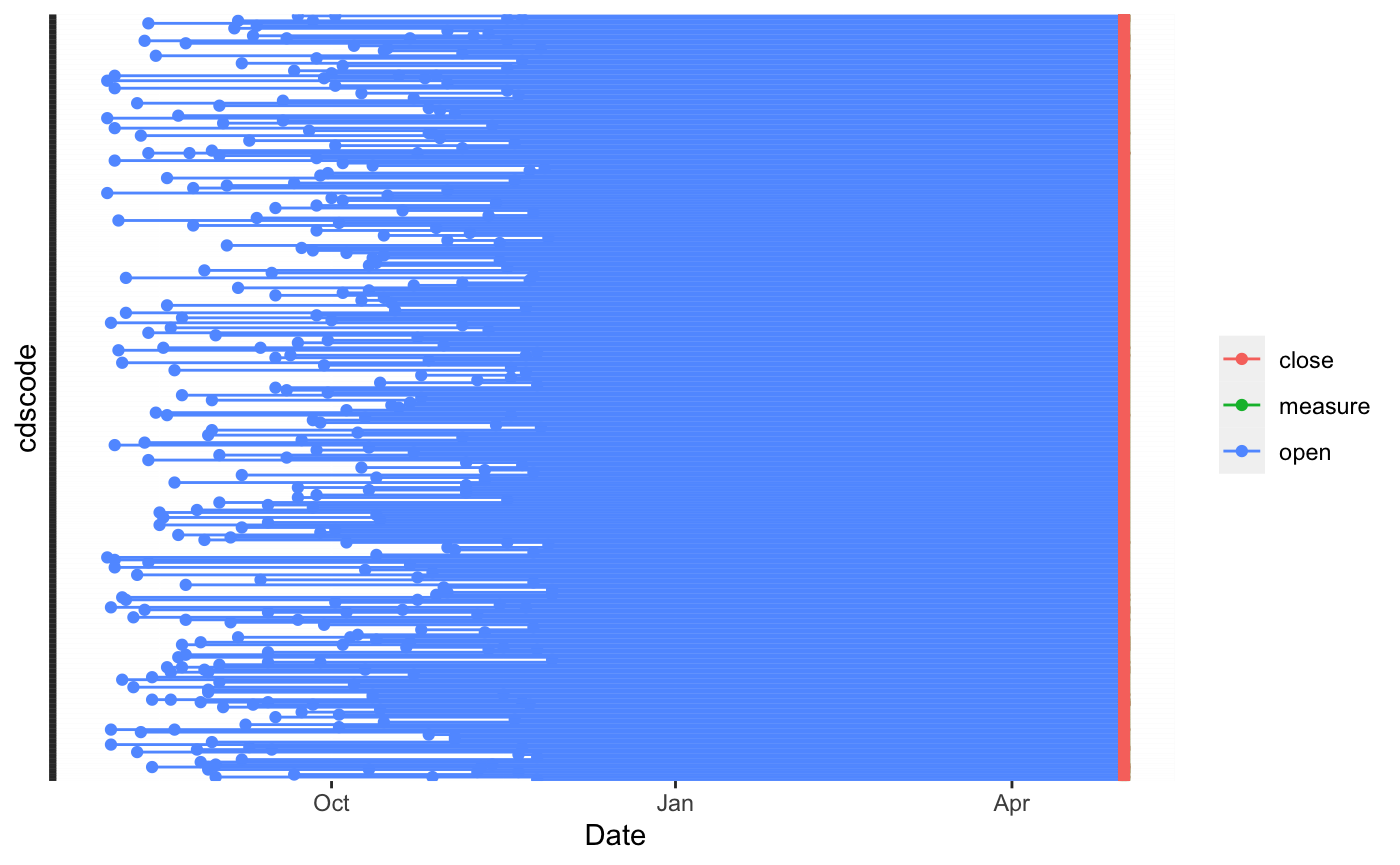
To finish off this section we’ll highlight a timeline plot that is currently available for visualizing the temporal exposure for subjects. The plot below shows when the different schools opened and closed. Since we’re showing all schools were closed and measured at the same time, we have a uniform line at the right side. This is just a feature of how we constructed the data, but it could be different. As the starting times show variability on the left hand side of the plot, it is not hard to imagine a setting in which there’d be similar variability for closing and measure times.
plot(bdf,'time')
Summary
This vignette demonstrated how to construct benvos iteratively using raw location and temporal data of subject and BEFs as well as how to manipulate and display the constructed data. We also showed a quick example highlighting how these objects are used in other packages, like rsstap, to understand how BEF’s may impact human health in a sample analysis using data that can be accessed publicly from the internet. It is my hope that this package makes working with the very particular relational structure of built environment data, easier and more accessible for those interested in studying it.