Introduction
This vignette serves to introduce the philosophy and structure of the rbenvo package, which implements the benvo class where benvo standards for Built Environment Object. This class makes working with built environment data easier by offering a convenient interface and methods for working with this type of relational data. We’ll illustrate some of the very basics of how to use benvo’s in this vignette as well as give some references as to how it might be used in other packages or settings.
We’ll begin by loading the library and the two example data sets involving subjects living near Fast Food Restaurants (FFR). One of the two data sets will be for the subject level information, FFR_subjects, the other contains some measure of exposure (Distance/Time) that describe how long and/or how close subjects are located near the Built Environment Features (BEFs).
The subject dataframe should look familiar. This is a tidy dataset with an ID and two subject-level measures: BMI and sex.
head(FFR_subjects,5)
#> # A tibble: 5 x 3
#>      id   BMI   sex
#>   <int> <dbl> <int>
#> 1     1  28.9     1
#> 2     2  33.0     1
#> 3     3  46.9     0
#> 4     4  30.2     1
#> 5     5  43.3     0
The distance dataframe is a tidy “long” dataframe, containing multiple nearby BEF exposures per subject. Note that there must be at least two columns in every BEF dataset added to a benvo. One for the id and one for the Distance/Time data measured. Additionally, the latter columns must be named as “Distance” or “Time”,as benvo’s use these titles to perform their methods.
head(FFR_distances,5)
#> # A tibble: 5 x 2
#>      id Distance
#>   <int>    <dbl>
#> 1     1    0.773
#> 2     1    0.734
#> 3     1    0.997
#> 4     1    0.470
#> 5     1    0.523
In order to create a benvo we’ll pass the two dataframes to the benvo() function, wrapping the FFR_distances data frame in a list.
bdf <- benvo(subject_data = FFR_subjects,
             sub_bef_data = list(FFR=FFR_distances),by='id')
summary(bdf)
#> Subject Data:
#> ---------------------------:
#> Observations:  1000
#> Columns:  3
#>
#> BEF Data:
#> ---------------------------:
#> Number of Features:  1
#> Features:
#>   Name Measures
#> 1  FFR Distance
And that’s it! That’s all it takes to create a benvo, which is very particular kind of wrapper function for handling this specific kind of relational data in which there is a one-to-many relationship between the subject data frame and each BEF data frame.
Benvo Methods
While the summary method above gives us a look at the overall benvo object, if we simply print the benvo, we’ll get a view of whatever data frame is active.
bdf
#> Active df:  subject
#> # A tibble: 1,000 x 3
#>       id   BMI   sex
#>    <int> <dbl> <int>
#>  1     1  28.9     1
#>  2     2  33.0     1
#>  3     3  46.9     0
#>  4     4  30.2     1
#>  5     5  43.3     0
#>  6     6  34.1     1
#>  7     7  35.2     1
#>  8     8  28.3     0
#>  9     9  43.2     0
#> 10    10  44.4     1
#> # … with 990 more rows
This notion of an active dataframe is inspired by (or borrowed from, depending on your perspective), the set-up of the tidygraph package which also has a particular kind of relational data structure.
Essentially, the active dataframe is that dataframe which is currently available for viewing and editing via the popular dplyr verbs.
bdf %>% activate(FFR) %>% filter(id<=5)
#> Active df:  FFR
#> # A tibble: 37 x 2
#>       id Distance
#>    <int>    <dbl>
#>  1     1    0.773
#>  2     1    0.734
#>  3     1    0.997
#>  4     1    0.470
#>  5     1    0.523
#>  6     2    0.369
#>  7     2    0.533
#>  8     2    0.779
#>  9     2    0.723
#> 10     2    0.375
#> # … with 27 more rows
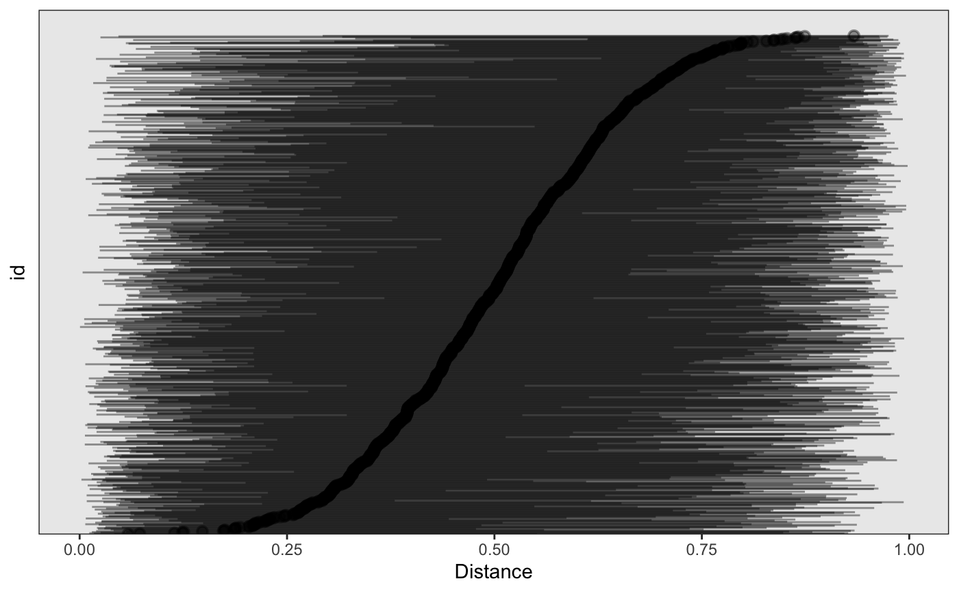
There are also a number of helpful plotting functions specific to built environment data built in, as one last descriptive offering, we can plot a point-range of the distances for each subject using the plot function and passing the BEF label we want plotted. You’ll see that there are several observations missing, since not every subject lives near a FFR.
plot(bdf)
#> Warning: Removed 49 rows containing missing values (geom_pointrange).
Other packages
While the above descriptive statistics are nice, the real power of using benvos is that they offer functions like joinvo to easily join the subject and bef data frames, which can be useful in setting up the data for models in other packages. Below we’ll use the joinvo function, passing the benvo and bef character label for which table we want joined.
joinvo(bdf,"FFR")
#> # A tibble: 9,550 x 2
#>       id Distance
#>    <int>    <dbl>
#>  1     1    0.773
#>  2     1    0.734
#>  3     1    0.997
#>  4     1    0.470
#>  5     1    0.523
#>  6     2    0.369
#>  7     2    0.533
#>  8     2    0.779
#>  9     2    0.723
#> 10     2    0.375
#> # … with 9,540 more rows
Similarly, it is often the case - in my work at least - that some sort of model involving both the built environment data and the subject level data is needed. This means that information is incorporated at the subject level. This could manifest in, for example, the construction of a subject design matrix. Below I’ll demonstrate how this works in a cross sectional as well as longitudinal framework, whilst highlighting how some of the previous functions take advantage of the longitudinal structure.
str(subject_design(bdf,BMI ~ sex))
#> List of 3
#>  $ y          : Named num [1:1000] 28.9 33 46.9 30.2 43.3 ...
#>   ..- attr(*, "names")= chr [1:1000] "1" "2" "3" "4" ...
#>  $ X          : num [1:1000, 1:2] 1 1 1 1 1 1 1 1 1 1 ...
#>   ..- attr(*, "dimnames")=List of 2
#>   .. ..$ : chr [1:1000] "1" "2" "3" "4" ...
#>   .. ..$ : chr [1:2] "(Intercept)" "sex"
#>   ..- attr(*, "assign")= int [1:2] 0 1
#>  $ model_frame:'data.frame': 1000 obs. of  2 variables:
#>   ..$ BMI: num [1:1000] 28.9 33 46.9 30.2 43.3 ...
#>   ..$ sex: int [1:1000] 1 1 0 1 0 1 1 0 0 1 ...
#>   ..- attr(*, "terms")=Classes 'terms', 'formula'  language BMI ~ sex
#>   .. .. ..- attr(*, "variables")= language list(BMI, sex)
#>   .. .. ..- attr(*, "factors")= int [1:2, 1] 0 1
#>   .. .. .. ..- attr(*, "dimnames")=List of 2
#>   .. .. .. .. ..$ : chr [1:2] "BMI" "sex"
#>   .. .. .. .. ..$ : chr "sex"
#>   .. .. ..- attr(*, "term.labels")= chr "sex"
#>   .. .. ..- attr(*, "order")= int 1
#>   .. .. ..- attr(*, "intercept")= int 1
#>   .. .. ..- attr(*, "response")= int 1
#>   .. .. ..- attr(*, ".Environment")=<environment: R_GlobalEnv>
#>   .. .. ..- attr(*, "predvars")= language list(BMI, sex)
#>   .. .. ..- attr(*, "dataClasses")= Named chr [1:2] "numeric" "numeric"
#>   .. .. .. ..- attr(*, "names")= chr [1:2] "BMI" "sex"
Longitudinal Example
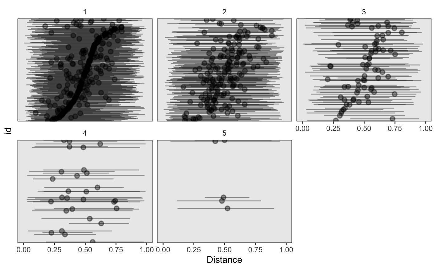
For our longitudinal example we’ll look at a dataset that imagines a hypothetical set of grocery or “Healthy Food Stores”(HFS) near subjects. Subjects or grocery stores may move over time so this will be reflected in our data. Below we’ll repeat the similar descriptives from above, highlighting the differences in a longitudinal benvo.
data("longitudinal_HFS")
longitudinal_HFS
#> Active df:  subject
#> # A tibble: 596 x 6
#>       id   sex subj_effect measurement exposure   BMI
#>    <int> <int>       <dbl>       <int>    <dbl> <dbl>
#>  1     1     0      0.0974           1    -4.27  28.1
#>  2     1     0      0.0974           2    -3.30  29.4
#>  3     1     0      0.0974           3    -5.72  29.7
#>  4     1     0      0.0974           4    -2.45  30.6
#>  5     2     1     -0.202            1    -3.15  28.0
#>  6     2     1     -0.202            2    -6.20  24.5
#>  7     3     1      0.0641           1    -2.77  28.2
#>  8     4     1     -0.0627           1    -2.61  27.4
#>  9     4     1     -0.0627           2    -3.19  26.9
#> 10     5     0      0.0980           1    -4.52  30.1
#> # … with 586 more rows
summary(longitudinal_HFS)
#> Subject Data:
#> ---------------------------:
#> Observations:  596
#> Columns:  6
#> Num Subjects:  1
#>
#> BEF Data:
#> ---------------------------:
#> Number of Features:  1
#> Features:
#>   Name      Measures
#> 1  HFS Distance-Time
plot(longitudinal_HFS,
     plotfun = "pointrange",
     term ="HFS",
     component = "Distance",
     p = 0.9)
#> Warning: Removed 24 rows containing missing values (geom_pointrange).
Analogous to subject_design there is also the longitudinal_design function which effectively allows for lme4 style formulas to be used, incorporating subject or group level effects from the subject_data in the benvo and returning a glmod object along with the corresponding X and y design matrix and outcome vector, respectively.
str(longitudinal_design(longitudinal_HFS,BMI ~ sex + (1|id)),max.level=1)
#> List of 3
#>  $ y    : num [1:596] 28.1 29.4 29.7 30.6 28 ...
#>  $ X    : num [1:596, 1:2] 1 1 1 1 1 1 1 1 1 1 ...
#>   ..- attr(*, "dimnames")=List of 2
#>   ..- attr(*, "assign")= int [1:2] 0 1
#>   ..- attr(*, "msgScaleX")= chr(0)
#>  $ glmod:List of 6
Further Information
This completes this preliminary introduction to the rbenvo package. For current uses please see the rsstap or rstapDP packages. I’ve found that having these data structures greatly simplifies my code and allows for data to be organized more easily. If you’re working with similar data, I hope you find the same!